Installation and Examples

Installation and Examples#

Installation#

AcATaMa is available from the official QGIS Plugin Repository. To install it:

Open QGIS and go to Plugins → Manage and Install Plugins….
In the search bar, type AcATaMa and click Install Plugin.
Once installed, activate the plugin via the Plugins menu or Plugins toolbar.

External Python libraries#

AcATaMa uses Dask for parallel raster pixel counting. These Python libraries are distributed as a separate extlibs.zip release asset instead of being bundled in the plugin package.

When the plugin starts and Dask is not available, AcATaMa downloads extlibs.zip from the matching GitHub release and extracts it into the QGIS profile plugin folder. If the computer is offline, download extlibs.zip manually from the same release as the installed plugin and extract its contents into QGIS3/profiles/default/python/plugins/AcATaMa/extlibs.

Examples#

Note

Download the examples in order to load them in Acatama and explore the configuration and results, you can find the zip here

Note

Load the examples using the Restore configuration function in AcATaMa. The examples are already fully configured and completed, so you can explore all settings and results as a reference for your own configuration.

The examples were made with the forest land change map in Colombia for the year 2019-2020, the study area is the Tinigua National Natural Park an area with a high deforestation rate that is located on the border of the Colombian Amazon and the Andes mountains. The classes that are assessed in this thematic accuracy assessment are Stable Forest, Non-Stable Forest, and Deforestation.

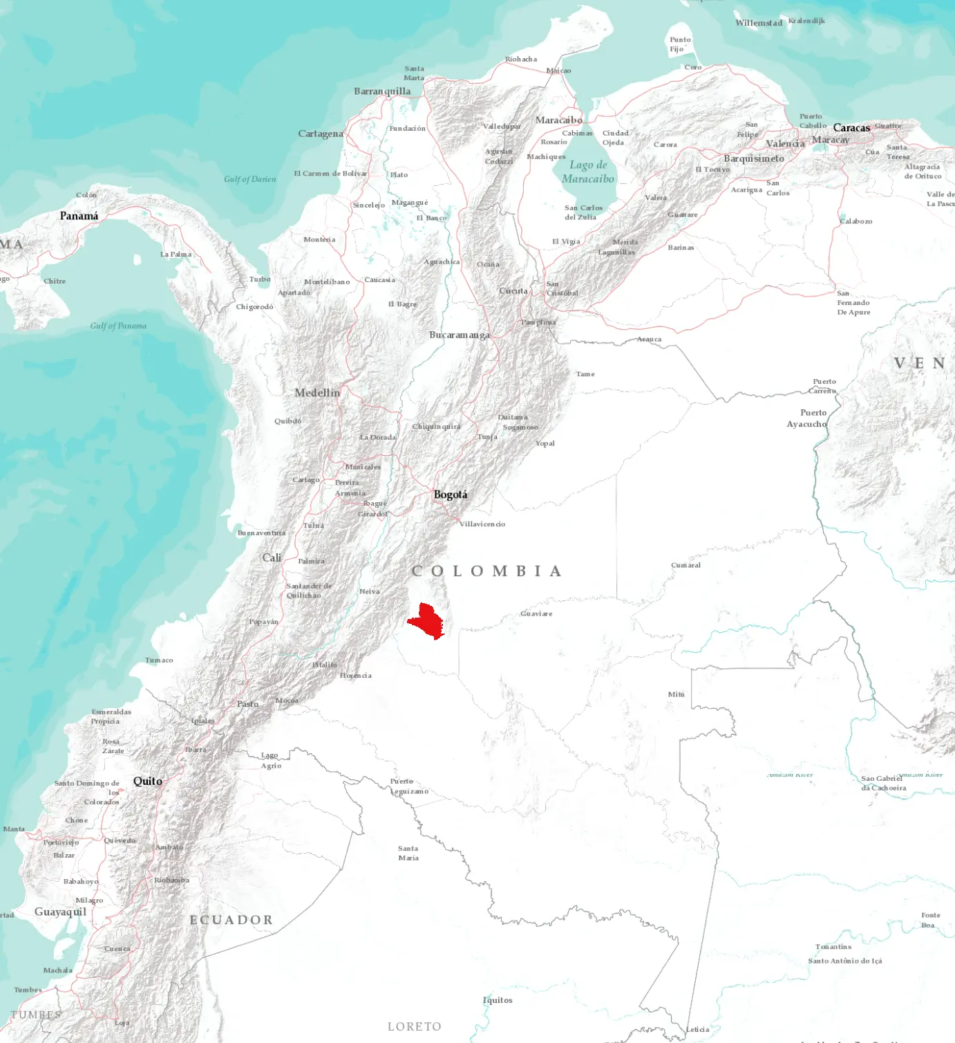
The three types of sampling were carried out: simple random, systematic and stratified. For each sampling, 500 evaluation points were chosen and Landsat images from 2019 and 2020 were used as reference data to identify the change in coverage. The Landsat satellite images are the primary input for evaluating thematic accuracy, and they are supplemented by a query of satellite image data from the Google Earth platform (not set in the examples, however we recommend having supplemental data by Google Earth Engine plugin based on your use case and needs)

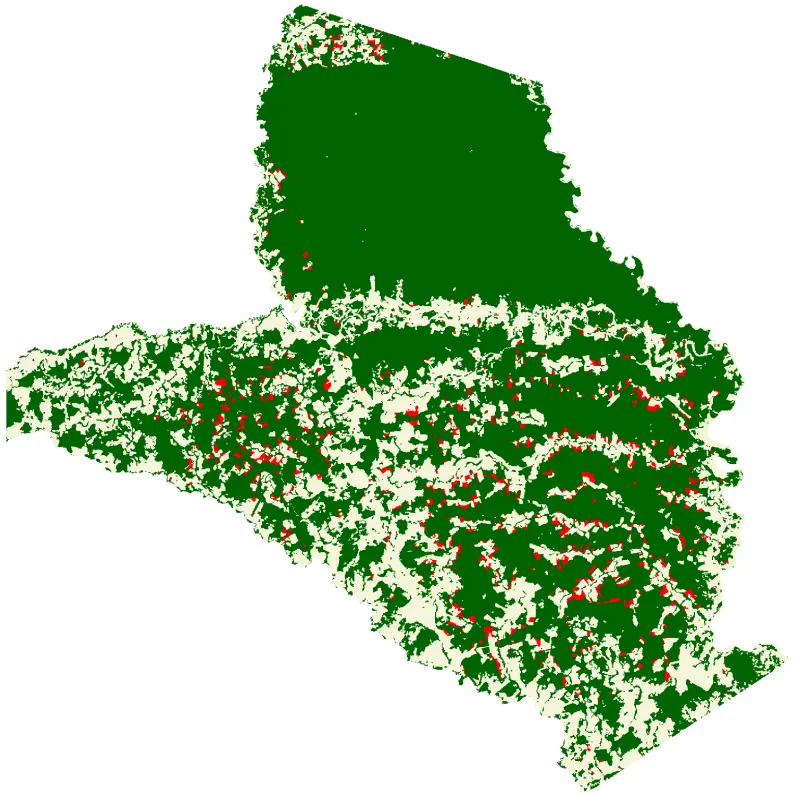
The main goal of these exercises is to define the agreement between the forest change detection map and the manual classification by visually interpreting the reference data, which will result in an error matrix expressed in terms of the area relationship. The following table summarizes the response protocol specifications for all the exercises proposed:

Protocol specifications	Description
Reference Data	Landsat 2019, 2020 and Google Earth images.
Evaluation protocol	One hectare is designated as a sampling unit, that is, 3x3 pixels
labeling protocol	They are classified into four classes: · Stable forest · Non stable forest · Deforestation · As a labeling rule: if there is doubt about the pixel classification, the dominant class in the 9 neighboring pixels should be chosen.

Finally, the results that are obtained when the sampling points are completed. This example presents the results with the different estimators, associated with the types of sampling such as simple random, systematic, stratified and post-stratified.

Important

All files in this example are for demonstration purposes only and do not represent official/real data.

Real-World Case Study#

A complete, peer-reviewed application of the full AcATaMa workflow assessed the accuracy of Colombia’s National Forest Change Map for 2018–2019 [Llano et al., 2026] — a 30 × 30 m national raster product with four classes (stable forest, non-stable forest, deforestation, and no information).

It used a stratified random design with a total sample size of n = 10,010, a fixed allocation of 1,000 samples to the rare deforestation stratum, a target overall standard error of 0.003, and a fixed seed for reproducibility. The overall accuracy was 94.9 %, and the result shows the practical value of sample-based area estimation: the map classified 158,900 ha as deforestation, whereas the accuracy-adjusted estimate was 142,588 ± 25,002 ha — a reduction of roughly 10.3 % attributable to the correction of classification errors.